
Coarse-to-Fine CNN for Image Super-Resolution

Contributed by Chunwei Tian, Yong Xu, Wangmeng Zuo, Bob Zhang, Lunke Fei, Chia-Wen Lin, based on the IEEEXplore® article, “Coarse-to-Fine CNN for Image Super-Resolution”, published in the IEEE Transactions on Multimedia, 2020.
Guide
Digital imaging devices are often affected by shooting environment, i.e., weather, hardware quality and camera shake, which will result in low-quality image of collected images. To address these problem, deep learning techniques use end-to-end architectures to learn low-resolution to high-resolution mappings [1,2]. Most of existing methods use upsampling operations in the end of networks to amplify predicted low-frequency features, which may result in unstable training. To overcome this challenge, we use hierarchical information of high- and low- frequency information to gather complementary contextual information, which can effectively overcome the problem. More information of this paper can be obtained from the article. Codes of CFSRCNN is accessible on GitHub.
The Proposed Method
As shown in Figs. 1 and 2, our proposed CFSRCNN [3] is composed of a stack of Feature Extraction Blocks (FEBs), an Enhancement Block (EB), a Construction Block (CB) and a Feature Refinement Block (FRB). The combination of the stacked FEBs, EB and CB can make use of hierarchical LR features extracted from the LR image with fewer parameters to enhance obtained LR features and derive coarse SR features. Specifically, combining an FEU and a CU into an FEB obtains long- and short-path features. Also, fusing the obtained features via the two closest FEUs can enlarge the effects of shallow layers on deep layers to improve the representing power of the SR model. The CU can distill more useful information and reduce the number of parameters. The EB fuses the features of all FEUs to offer complementary features for the stacked FEBs and prevent from the loss of edge information caused by the repeated distillation operations. Gathering several extra stacked FEUs into the EB removes over-enhanced pixel points from the previous stage of the EB. After that, the CB utilizes the global and local LR features to obtain coarse SR features. Finally, the FRB utilizes HR features to more effectively learn HR features and reconstruct a HR image. We introduce these techniques in the later sections.
The proposed CFSRCNN is different from existing methods. The specific differences are listed as following.
- Prevalent super-resolution methods such as residual dense network (RDN), channel-wise and spatial feature modulation (CSFM), as shown in Fig. 3, consider each layer as input to all subsequent layers, which greatly increases the training time. The FEBs only fuse the adjacent output features of FEB to enhance the last obtained low-resolution features. In addition, the use of heterogeneous convolutions composed of 3x3 and 1x1 instead of stacked 3x3 convolutions significantly reduces the network depth, complexity and running time without sacrificing visual quality (CFSRCNN parameters are only 5.5% of RDB and 9.3% of CSFM). In addition, heterogeneous convolutions composed of 3x3 and 1x1 replace the stacked 3x3 convolutions, which significantly reduces the network depth, complexity and running time without sacrificing visual quality (CFSRCNN parameters are only 5.5% of RDB and 9.3% of CSFM).
- Residual learning techniques are embedded into EB and replaces the popular concertante operation, which complements FEBs to enhance the robustness of obtaining LR features. To prevent over-enhancement of image pixels, stacking multiple layers is used to smooth the obtained LR features.
- The combination of global and local features using residual learning and upsampling operations prevents the loss of LR features due to sudden pixel scaling. And the FRB smooths the training process and extract more accurate SR features.
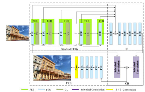
Figure 1. Network architecture of CFSRCNN
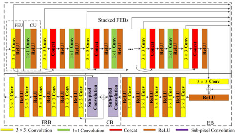
Figure 2. Network architecture of CFSRCNN
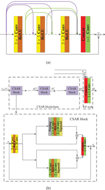
Figure 3. (a) The residual dense block (RDB) architecture; (b) The FMM module in the CFSM
Contributions
- We propose a cascaded network that combines LR and HR features to prevent possible training instability and performance degradation caused by upsampling operations.
- We propose a novel feature fusion scheme based on heterogeneous convolutions to well resolve the long-term dependency problem and prevent information loss so as to significantly improve the efficiency of SISR without sacrificing the visual quality of reconstructed SR images.
- The proposed network achieves both good performance and high computational efficiency for SISR.
Experimental Results
To demonstrate the effectiveness of our method, we test our method on Set5, Set14, B100 and U100 as shown in Tables 1,2, 3 and 4. Our method has surpassed popular image super-resolution methods, i.e., CSCN and DnCNN. Although the performance of our method is slightly inferior to that of RDN, CSFM, etc. in Table 7, our method has less complexity and faster denoising time in Tables 5 and 6. To observe visual effects, we choose an area of predicted images as observation area. If observation area is clearer, its effect is better. As shown in Fig. 4 and 5, we can see that our method is clearer than that other superinsulation methods. According to mentioned illustrations, our method is more effective for image super-resolution.
Table 1. Comparison of average PSNR/SSIM performances for ×2, ×3, and ×4 upscaling on Set5.
| Dataset | Model | ×2 | ×3 | ×4 |
| PSNR/SSIM | PSNR/SSIM | PSNR/SSIM | ||
| Set 5 | Bicubic | 33.66/0.9299 | 30.39/0.8682 | 28.42/0.8104 |
| A+ | 36.54/0.9544 | 32.58/0.9088 | 30.28/0.8603 | |
| RFL | 36.54/0.9537 | 32.43/0.9057 | 30.14/0.8548 | |
| SelfEx | 36.49/0.9537 | 32.58/0.9093 | 30.31/0.8619 | |
| CSCN | 36.93/0.9552 | 33.10/0.9144 | 30.86/0.8732 | |
| RED30 | 37.66/0.9599 | 33.82/0.9230 | 31.51/0.8869 | |
| DnCNN | 37.58/0.9590 | 33.75/0.9222 | 31.40/0.8845 | |
| TNRD | 36.86/0.9556 | 33.18/0.9152 | 30.85/0.8732 | |
| FDSR | 37.40/0.9513 | 33.68/0.9096 | 31.28/0.8658 | |
| SRCNN | 36.66/0.9542 | 32.75/0.9090 | 30.48/0.8628 | |
| FSRCNN | 37.00/0.9558 | 33.16/0.9140 | 30.71/0.8657 | |
| RCN | 37.17/0.9583 | 33.45/0.9175 | 31.11/0.8736 | |
| VDSR | 37.53/0.9587 | 33.66/0.9213 | 31.35/0.8838 | |
| DRCN | 37.63/0.9588 | 33.82/0.9226 | 31.53/0.8854 | |
| CNF | 37.66/0.9590 | 33.74/0.9226 | 31.55/0.8856 | |
| LapSRN | 37.52/0.9590 | - | 31.54/0.8850 | |
| IDN | 37.83/0.9600 | 34.11/0.9253 | 31.82/0.8903 | |
| DRRN | 37.74/0.9591 | 34.03/0.9244 | 31.68/0.8888 | |
| BTSRN | 37.75/- | 34.03/- | 31.85/- | |
| MemNet | 37.78/0.9597 | 34.09/0.9248 | 31.74/0.8893 | |
| CARN-M | 37.53/0.9583 | 33.99/0.9236 | 31.92/0.8903 | |
| CARN | 37.76/0.9590 | 34.29/0.9255 | 32.13/0.8937 | |
| EEDS+ | 37.78/0.9609 | 33.81/0.9252 | 31.53/0.8869 | |
| TSCN | 37.88/0.9602 | 34.18/0.9256 | 31.82/0.8907 | |
| DRFN | 37.71/0.9595 | 34.01/0.9234 | 31.55/0.8861 | |
| RDN | 38.24/0.9614 | 34.71/0.9296 | 32.47/0.8990 | |
| CSFM | 38.26/0.9615 | 34.76/0.9301 | 32.61/0.9000 | |
| SRFBN | 38.11/0.9609 | 34.70/0.9292 | 32.47/0.8983 | |
| CFSRCNN(Ours) | 37.79/0.9591 | 34.24/0.9256 | 32.06/0.8920 |
Table 2. Comparison of average PSNR/SSIM performances for ×2, ×3, and ×4 upscaling on Set14.
| Dataset | Model | ×2 | ×3 | ×4 |
| PSNR/SSIM | PSNR/SSIM | PSNR/SSIM | ||
| Set14 | Bicubic | 30.24/0.8688 | 27.55/0.7742 | 26.00/0.7027 |
| A+ | 32.28/0.9056 | 29.13/0.8188 | 27.32/0.7491 | |
| RFL | 32.26/0.9040 | 29.05/0.8164 | 27.24/0.7451 | |
| SelfEx | 32.22/0.9034 | 29.16/0.8196 | 27.40/0.7518 | |
| CSCN | 32.56/0.9074 | 29.41/0.8238 | 27.64/0.7578 | |
| RED30 | 32.94/0.9144 | 29.61/0.8341 | 27.86/0.7718 | |
| DnCNN | 33.03/0.9128 | 29.81/0.8321 | 28.04/0.7672 | |
| TNRD | 32.51/0.9069 | 29.43/0.8232 | 27.66/0.7563 | |
| FDSR | 33.00/0.9042 | 29.61/0.8179 | 27.86/0.7500 | |
| SRCNN | 32.42/0.9063 | 29.28/0.8209 | 27.49/0.7503 | |
| FSRCNN | 32.63/0.9088 | 29.43/0.8242 | 27.59/0.7535 | |
| RCN | 32.77/0.9109 | 29.63/0.8269 | 27.79/0.7594 | |
| VDSR | 33.03/0.9124 | 29.77/0.8314 | 28.01/0.7674 | |
| DRCN | 33.04/0.9118 | 29.76/0.8311 | 28.02/0.7670 | |
| CNF | 33.38/0.9136 | 29.90/0.8322 | 28.15/0.7680 | |
| LapSRN | 33.08/0.9130 | 29.63/0.8269 | 28.19/0.7720 | |
| IDN | 33.30/0.9148 | 29.99/0.8354 | 28.25/0.7730 | |
| DRRN | 33.23/0.9136 | 29.96/0.8349 | 28.21/0.7720 | |
| BTSRN | 33.20/- | 29.90/- | 28.20/- | |
| MemNet | 33.28/0.9142 | 30.00/0.8350 | 28.26/0.7723 | |
| CARN-M | 33.26/0.9141 | 30.08/0.8367 | 28.42/0.7762 | |
| CARN | 33.52/0.9166 | 30.29/0.8407 | 8.60/0.7806 | |
| EEDS+ | 33.21/0.9151 | 29.85/0.8339 | 28.13/0.7698 | |
| TSCN | 33.28/0.9147 | 29.99/0.8351 | 28.28/0.7734 | |
| DRFN | 33.29/0.9142 | 30.06/0.8366 | 28.30/0.7737 | |
| RDN | 34.01/0.9212 | 30.57/0.8468 | 28.81/0.7871 | |
| CSFM | 34.07/0.9213 | 30.63/0.8477 | 28.87/0.7886 | |
| SRFBN | 33.82/0.9196 | 30.51/0.8461 | 28.81/0.7868 | |
| CFSRCNN (Ours) | 33.51/0.9165 | 30.27/0.8410 | 28.57/0.7800 |
Table 3. Comparison of average PSNR/SSIM performances for ×2, ×3, and ×4 upscaling on B100.
| Dataset | Model | ×2 | ×3 | ×4 |
| PSNR/SSIM | PSNR/SSIM | PSNR/SSIM | ||
| B100 | Bicubic | 29.56/0.8431 | 27.21/0.7385 | 25.96/0.6675 |
| A+ | 31.21/0.8863 | 28.29/0.7835 | 26.82/0.7087 | |
| RFL | 31.16/0.8840 | 28.22/0.7806 | 26.75/0.7054 | |
| SelfEx | 31.18/0.8855 | 28.29/0.7840 | 26.84/0.7106 | |
| CSCN | 31.40/0.8884 | 28.50/0.7885 | 27.03/0.7161 | |
| RED30 | 31.98/0.8974 | 28.92/0.7993 | 27.39/0.7286 | |
| DnCNN | 31.90/0.8961 | 28.85/0.7981 | 27.29/0.7253 | |
| TNRD | 31.40/0.8878 | 28.50/0.7881 | 27.00/0.7140 | |
| FDSR | 31.87/0.8847 | 28.82/0.7797 | 27.31/0.7031 | |
| SRCNN | 31.36/0.8879 | 28.41/0.7863 | 26.90/0.7101 | |
| FSRCNN | 31.53/0.8920 | 28.53/0.7910 | 26.98/0.7150 | |
| VDSR | 31.90/0.8960 | 28.82/0.7976 | 27.29/0.7251 | |
| DRCN | 31.85/0.8942 | 28.80/0.7963 | 27.23/0.7233 | |
| CNF | 31.91/0.8962 | 28.82/0.7980 | 27.32/0.7253 | |
| LapSRN | 31.80/0.8950 | - | 27.32/0.7280 | |
| IDN | 32.08/0.8985 | 28.95/0.8013 | 27.41/0.7297 | |
| DRRN | 32.05/0.8973 | 28.95/0.8004 | 27.38/0.7284 | |
| BTSRN | 32.05/- | 28.97/- | 27.47/- | |
| MemNet | 32.08/0.8978 | 28.96/0.8001 | 27.40/0.7281 | |
| CARN-M | 31.92/0.8960 | 28.91/0.8000 | 27.44/0.7304 | |
| CARN | 32.09/0.8978 | 29.06/0.8034 | 27.58/0.7349 | |
| EEDS+ | 31.95/0.8963 | 28.88/0.8054 | 27.35/0.7263 | |
| TSCN | 32.09/0.8985 | 28.95/0.8012 | 27.42/0.7301 | |
| DRFN | 32.02/0.8979 | 28.93/0.8010 | 27.39/0.7293 | |
| RDN | 32.34/0.9017 | 29.26/0.8093 | 27.72/0.7419 | |
| CSFM | 32.37/0.9021 | 29.30/0.8105 | 27.76/0.7432 | |
| SRFBN | 32.29/0.9010 | 29.24/0.8084 | 27.72/0.7409 | |
| CFSRCNN (Ours) | 32.11/0.8988 | 29.03/0.8035 | 27.53/0.7333 |
Table 4. Comparison of average PSNR/SSIM performances for ×2, ×3, and ×4 upscaling on U100.
| Dataset | Model | ×2 | ×3 | ×4 |
| PSNR/SSIM | PSNR/SSIM | PSNR/SSIM | ||
| U100 | Bicubic | 26.88/0.8403 | 24.46/0.7349 | 23.14/0.6577 |
| A+ | 29.20/0.8938 | 26.03/0.7973 | 24.32/0.7183 | |
| RFL | 29.11/0.8904 | 25.86/0.7900 | 24.19/0.7096 | |
| SelfEx | 29.54/0.8967 | 26.44/0.8088 | 24.79/0.7374 | |
| RED30 | 30.91/0.9159 | 27.31/0.8303 | 25.35/0.7587 | |
| DnCNN | 30.74/0.9139 | 27.15/0.8276 | 25.20/0.7521 | |
| TNRD | 29.70/0.8994 | 26.42/0.8076 | 24.61/0.7291 | |
| FDSR | 30.91/0.9088 | 27.23/0.8190 | 25.27/0.7417 | |
| SRCNN | 29.50/0.8946 | 26.24/0.7989 | 24.52/0.7221 | |
| FSRCNN | 29.88/0.9020 | 26.43/0.8080 | 24.62/0.7280 | |
| VDSR | 30.76/0.9140 | 27.14/0.8279 | 25.18/0.7524 | |
| DRCN | 30.75/0.9133 | 27.15/0.8276 | 25.14/0.7510 | |
| LapSRN | 30.41/0.9100 | - | 25.21/0.7560 | |
| IDN | 31.27/0.9196 | 27.42/0.8359 | 25.41/0.7632 | |
| DRRN | 31.23/0.9188 | 27.53/0.8378 | 25.44/0.7638 | |
| BTSRN | 31.63/- | 27.75/- | 25.74/- | |
| MemNet | 31.31/0.9195 | 27.56/0.8376 | 25.50/0.7630 | |
| CARN-M | 31.23/0.9193 | 27.55/0.8385 | 25.62/0.7694 | |
| CARN | 31.92/0.9256 | 28.06/0.8493 | 26.07/0.7837 | |
| TSCN | 31.29/0.9198 | 27.46/0.8362 | 25.44/0.7644 | |
| DRFN | 31.08/0.9179 | 27.43/0.8359 | 25.45/0.7629 | |
| RDN | 32.89/0.9353 | 28.80/0.8653 | 26.61/0.8028 | |
| CSFM | 33.12/0.9366 | 28.98/0.8681 | 26.78/0.8065 | |
| SRFBN | 32.62/0.9328 | 28.73/0.8641 | 26.60/0.8015 | |
| CFSRCNN (Ours) | 32.07/0.9273 | 28.04/0.8496 | 26.03/0.7824 |
Table 5. Comparison of run-time(seconds) of various SR methods on HR images of sizes 256x256, 512x512 and 1024x1024 for x2 Upscaling.
| Single Image Super-Resolution | |||
| Size | 256×256 | 512×512 | 1024×1024 |
| VDSR | 0.0172 | 0.0575 | 0.2126 |
| DRRN | 3.063 | 8.050 | 25.23 |
| MemNet | 0.8774 | 3.605 | 14.69 |
| RDN | 0.0553 | 0.2232 | 0.9124 |
| SRFBN | 0.0761 | 0.2508 | 0.9787 |
| CARN-M | 0.0159 | 0.0199 | 0.0320 |
| CFSRCNN (Ours) | 0.0153 | 0.0184 | 0.0298 |
Table 6. Comparison of model complexities of various SR methods for x2 upscaling.
| Methods | Parameters | Flops |
| VDSR | 665K | 15.82G |
| DnCNN | 556K | 13.20G |
| DRCN | 1,774K | 42.07G |
| MemNet | 677K | 16.06G |
| CARN-M | 412K | 2.50G |
| CARN | 1,592K | 10.13G |
| CSFM | 12,841K | 76.82G |
| RDN | 21,937K | 130.75G |
| SRFBN | 3,631K | 22.24G |
| CFSRCNN (Ours) | 1,200K | 11.08G |
Table 7. Comparison of average PSNR/SSIM performances of various SR methods for ×2, ×3, and ×4 upscaling on 720P.
| Dataset | Model | ×2 | ×3 | ×4 |
| PSNR/SSIM | PSNR/SSIM | PSNR/SSIM | ||
| 720p | CARN-M | 43.62/0.9791 | 39.87/0.9602 | 37.61/0.9389 |
| CARN | 44.57/0.9809 | 40.66/0.9633 | 38.03/0.9429 | |
| CFSRCNN (Ours) | 44.77/0.9811 | 40.93/0.9656 | 38.34/0.9482 |

Figure 4. Visual qualitative comparison of various SR methods for ×2 upscaling on Set14: (a) HR image (PSNR/SSIM), (b) Bicubic (26.85/0.9468), (c) SRCNN (30.24/0.9743), (d) SelfEx (31.49/0.9823), (e) CARN-M (33.63/0.9888) and (f) CFSRCNN (34.45/0.9901).
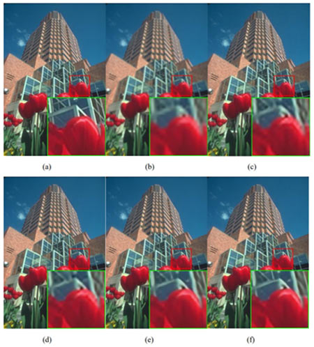
Figure 5. Subjective visual quality comparison of various SR methods for ×3 upscaling on B100: (a) HR image (PSNR/SSIM), (b) Bicubic (25.52/0.7731), (c) SRCNN (26.58/0.8217), (d) SelfEx (27.32/0.8424), (e) CARN-M (27.90/0.8626) and (f) CFSRCNN (28.56/0.8732).
Conclusion
In this paper, we proposed a coarse-to-fine super-resolution CNN (CFSRCNN) for single-image super-resolution. CFSRCNN combines low-resolution and high-resolution features by cascading several types of modular blocks to prevent possible training instability and performance degradation caused by upsampling operations. We have also proposed a novel feature fusion scheme based on heterogeneous convolutions to address the long-term dependency problem as well as prevent information loss so as to significantly improve the computational efficiency of super-resolution without sacrificing the visual quality of reconstructed images. Comprehensive evaluations on four benchmark datasets demonstrate that CFSRCNN offers an excellent trade-off among visual quality, computational efficiency, and model complexity. In this paper, we proposed a coarse-to-fine super-resolution CNN (CFSRCNN) for single-image super-resolution. CFSRCNN combines low-resolution and high-resolution features by cascading several types of modular blocks to prevent possible training instability and performance degradation caused by up-sampling operations. We have also proposed a novel feature fusion scheme based on heterogeneous convolutions to address the long-term dependency problem as well as prevent information loss so as to significantly improve the computational efficiency of super-resolution without sacrificing the visual quality of reconstructed images. Comprehensive evaluations on four benchmark datasets demonstrate that CFSRCNN offers an excellent trade-off among visual quality, computational efficiency, and model complexity.
References:
[1] C. Dong, C. C. Loy, and X. Tang, “Accelerating the super-resolution convolutional neural network,” in Proc. Eur. Conf. Comput. Vision Springer,2016, pp. 391–407, doi: https://doi.org/10.1016/j.procs.2019.12.069.
[2] N. Ahn, B. Kang and K. -A. Sohn, "Image Super-Resolution via Progressive Cascading Residual Network," 2018 IEEE/CVF Conference on Computer Vision and Pattern Recognition Workshops (CVPRW), Salt Lake City, UT, USA, 2018, pp. 904-9048, doi: https://dx.doi.org/10.1109/CVPRW.2018.00123.
[3] C. Tian, Y. Xu, W. Zuo, B. Zhang, L. Fei and C. -W. Lin, "Coarse-to-Fine CNN for Image Super-Resolution," in IEEE Transactions on Multimedia, vol. 23, pp. 1489-1502, 2021, doi: https://dx.doi.org/10.1109/TMM.2020.2999182.