
Estimation in Multi-Object State Space Model
Contributed by Dr. Ba-Ngu Vo, based on the IEEEXplore® article, The Gaussian Mixture Probability Hypothesis Density Filter, and webinar, "Bayesian Multi-object Tracking: Probability Hypothesis Density Filter & Beyond."
State space model (SSM) is a fundamental concept in system theory that permeated through many fields of study. The 1990s witnessed a significant development in SSM with Mahler’s generalization of vector-valued state to finite set-valued state to accommodate multi-object systems [3], [6]. These systems arise from a host of multiple object tracking (MOT) applications where the number of objects and their states are unknown and vary randomly with time. This article provides a brief introduction to estimation in multi-object system.
State Estimation: In an SSM (or hidden Markov model), the system state is characterized by a vector in a state space X, see Fig. 1. The state xk ∈ X at time k, evolves from its previous value xk-1 ∈ X, and generates an observation vector zk in an observation space Z, according to the system equations
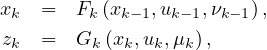
where Fk and Gk are non-linear mappings, uk (and uk-1) is the control signal, νk-1 and μk are, respectively, process and measurement noise.

Fig. 1. State Space Model (SSM).
State estimation is a fundamental problem in SSM, where the aim is to estimate the state trajectory x0:k ≜ (x0,...,xk). This can be achieved via smoothing, i.e., jointly estimating the history of the states, or via filtering, i.e., sequentially estimating the state at each time [1], [7], see Fig. 2. Jointly estimating the state history x0:k is intractable because the dimension of the variables (and hence computational load) per time step increases with k [7]. In practice, we need algorithms with fixed computational complexity per time step [7], hence it is imperative to smooth over short windows and link the estimates between the windows together. Filtering–the special case with a window length of one - is most widely used [1], [7].

Fig. 2. The state history x0:k = (x0,...,xk) defines the trajectory. Thus, a trajectory estimate can be
obtained from a history of individual state estimates.
In the Bayesian paradigm, the system state is modeled as a random vector, and filtering amounts to propagating the filtering density - the probability density of the current state conditioned on all observations up-to the current time [1], [7] - as illustrated in Fig. 3. The state estimate is usually the mode/mean of the filtering density.

Fig. 3: Propagation of the filtering density pk
Multi-Object State Estimation: Replacing the system state and observation vectors by finite sets gives a multi-object SSM that accommodates multi-object systems [3], [6], see Fig. 4. Analogous to conventional SSMs, the multi-object state Xk ⊂ X at time k, evolves from its previous value Xk-1 ⊂ X, and generates an observation Zk ⊂ Z, according to the multi-object system equations

where Sk(Xk-1) is the set of states generated from Xk-1, Bk is the set of new states born independently from Xk-1, Dk(Xk) is the set of observations generated from Xk, and Kk is the set of false alarms, at time k.

Fig. 4. Multi-object SSM. The number of states and observations vary with time.
Existing objects may not be detected, false alarms-observations not originated from any objects-may occur,
and it is not known which observations originated from which states.
State estimation in multi-object SSM involves estimating the multi-object trajectory - the set of trajectories of the underlying objects. However, unlike conventional SSMs, multi-object trajectory estimation may not be possible with multi-object filtering, as illustrated in Fig. 5.

(a) Multi-object state history X0:k = (X0,..., Xk).

(b) Multi-object trajectory.
Fig. 5. Multi-object states and trajectory (note X0 = {} in this example).
The multi-object state history X0:k does not necessarily represent the multi-object trajectory.
Thus, a sequence of multi-object state estimates does not necessarily provide a multi-object trajectory estimate.
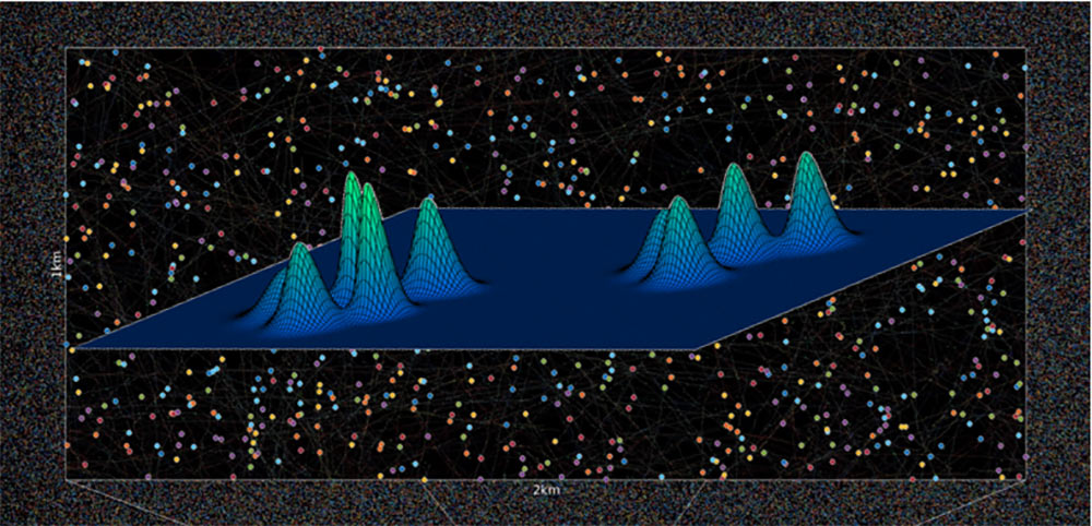
Under the Bayesian paradigm, the multi-object state is modeled as a random finite set (RFS), and filtering amounts to propagating the multi-object filtering density. The main challenge lies in the exponential complexity in the number of objects/observations. The widely-known Probability Hypothesis Density (PHD) filter alleviates the exponential complexity by propagating the PHD of the multi-object state in time [4], see Fig. 6. The PHD, or first-moment, of an RFS is a function on X, whose integral over any region S ⊆ X gives the expected number of object(s) in S. Thus, the PHD at x ∈ X is the instantaneous expected number of objects per unit hyper-volume. The PHD’s local maxima have highest local concentration of expected number of objects, and are the most likely locations of the objects. The PHD filter was also generalized to jointly propagate the PHD and cardinality distribution to improve cardinality estimation [5]. However, these filters (MATLAB codes) do not provide trajectory estimates.

Fig. 6. Propagation of the PHD. The integral of the PHD vk gives the expected number of objects,
and the peaks give the most likely locations of the objects.
Labeled Random Finite Set: To ensure that the multi-object trajectory is indeed the multi-object state history, the labeled RFS formulation augments distinct labels to individual states [3], [6], as illustrated in Fig. 7. Consequently, multi-object trajectory estimation can be accomplished via multi-object filtering [8]. Without labeling, there is no mechanism for linking trajectories from one window to another, even if these trajectories can be estimated over short windows. Hence, unlabeled multi-object trajectory estimation can only be performed with a growing window, which is infeasible even for a single trajectory [7].

Fig. 7. Labeled multi-object states and trajectory. The three objects are augmented with red, blue and white labels. Grouping the labeled states of X0:k according to labels (colors) gives the multi-object trajectory. Thus, analogous to conventional SSM,
a labeled multi-object trajectory estimate can be obtained from a history of labeled multi-object state estimates.
Generally, the multi-object smoother/filter propagates an intractably large weighted sum of functions. This can be approximated via parametric approximation, e.g. the PHD filter [4], or via truncating the sum, which requires that the truncated sum be a valid multi-object density, and quantification of the truncation error.
Apart from provision for trajectory estimation, labeled RFS ensures closure under truncation [8], and provides analytic truncation error [9], [11]. Further, this formulation admits an analytic solution known as the Generalized Labeled Multi-Bernoulli (GLMB) filter/smoother [8], [11], which can be implemented (MATLAB codes) with linear complexity in the:
- number of observations [10] (capable of tracking over a million objects [2], see Fig. 8);
- number of scans (for multi-object smoothing [11]);
- total number of observations across the sensors (for multi-sensor MOT [12]);
thereby, addressing the three key computational bottlenecks in MOT.

Fig. 8. GLMB filter tracking over 1 million objects simultaneously, under relatively challenging settings.
References:
[1] B. Anderson and J. Moore, Optimal Filtering, Prentice Hall, 1979.
[2] M. Beard, B.-T. Vo, and B.-N. Vo, “A Solution for Large-Scale Multi-Object Tracking,” IEEE Trans. Signal Processing, vol. 68, pp. 2754–2769, 2020, doi: 10.1109/TSP.2020.2986136.
[3] I. Goodman, R. Mahler, and H. Nguyen, Mathematics of Data Fusion. Kluwer Academic Publishers, 1997.
[4] R. Mahler, “Multitarget Bayes Filtering via first-order Multitarget Moments,” IEEE Trans. Aerosp. Electron. Syst., vol. 39, no. 4, pp. 1152–1178, 2003, doi: 10.1109/TAES.2003.1261119.
[5] R. Mahler, “PHD Filters of Higher order in Target Number,” IEEE Trans. Aerosp. Electron. Syst., vol. 43, no. 4, pp. 1523–1543, 2007, doi: 10.1109/TAES.2007.4441756.
[6] R. Mahler, Statistical Multisource-Multitarget Information Fusion, Artech House, 2007.
[7] S. Särkkä, Bayesian filtering and smoothing, Cambridge University Press, 2013.
[8] B.-T. Vo, and B.-N. Vo, “Labeled Random Finite Sets and multi-object conjugate priors,” IEEE Trans. Signal Process., vol. 61, no. 13, pp. 3460–3475, 2013, doi: 10.1109/TSP.2013.2259822.
[9] B.-N. Vo, B.-T. Vo, and D. Phung, "Labeled Random Finite Sets and the Bayes Multitarget Tracking Filter," IEEE Trans. Signal Process., vol. 62, no. 24, pp. 6554–6567, 2014, doi: 10.1109/TSP.2014.2364014.
[10] B.-N. Vo, B.-T. Vo, and H. Hoang, “An Efficient Implementation of the Generalized Labeled multi-Bernoulli Filter,” IEEE Trans. Signal Process., vol. 65, no. 8, pp. 1975–1987, 2017.
[11] B.-N. Vo, and B.-T. Vo. "A Multi-Scan Labeled Random Finite Set Model for Multi-object State Estimation," IEEE Trans. Signal Process., vol. 67, no. 19, pp. 4948–4963, 2019, doi: 10.1109/TSP.2019.2928953.
[12] B.-N. Vo, B.-T. Vo, and M. Beard, "Multi-Sensor Multi-Object Tracking with the Generalized Labeled Multi-Bernoulli Filter," IEEE Trans. Signal Process., vol. 67, no. 23, pp. 5952–5967, 2019, doi: 10.1109/TSP.2019.2946023.